Interact with Spatial data services using QGIS Desktop
QGIS is an open source desktop GIS application available for Windows, MacOX, Linux and Android. It supports a wide variety of spatial formats, spatial data services, digitisation tools and spatial processing tools. If you are not familiar with QGIS, follow the getting started tutorial first.
Visualize data using OGC:WMS
OGC:WMS visualizes data in a mapviewer. To display a WMS in QGIS, Select from the menu Layer > Add Layer > Add WMS/WMTS Layer. This opens the Add layer panel.
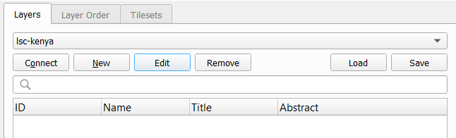
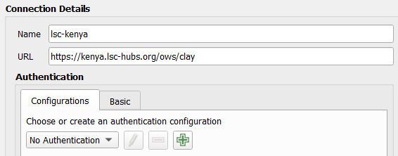
First we are adding a new service. Select the New button.
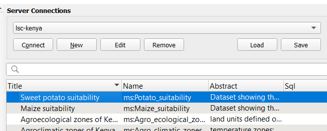
With the service selected, click the connect button and the layers available in the service are displayed
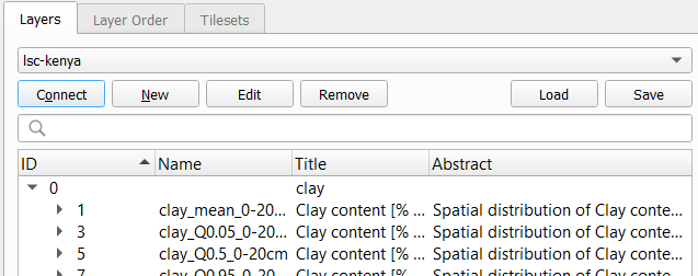
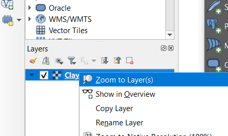
Select the relevant layer and click Add at the bottom of the panel. The Layer is now displayed on the map. If you don’t see it yet, right click the layer on the table of content and select Zoom to layer.
Understand that you can not select features, because the interaction with the service is based on images. You can however use the i tool to retrieve attribute information from pixels. A dedicated method on the service, called ‘getFeatureInfo’ is used.
Visualize and download vector data using OGC:WFS or OGCAPI:Features
OGC:WFS retrieves vector features from a dataset. OGCAPI:Features is a modern alternative to WFS, supported by some servers. Adding a WFS or Features layer to QGIS uses a similar procedure as adding a WMS layer. Select Layer > Add layer > Add WFS layer from the menu. Notice that only vector layers are shown, grid layers use the WCS protocol (see next paragraph).
Notice the build query button in the footer of the panel. This allows you to filter features on attribute value, for example pH < 5. Substantially less data will be retrieved, improving the performance.
With the layer added to the view, notice that the data has no styling, it acts as any other vector dataset. You can select features and even open the attribute table.
To extract a subset of the data, zoom to the area of interest, then right click the layer in the table of contents and select Export > Save Features As.
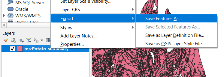
On the export panel, set the format, a file location and set the extent (current). Then select OK.
Visualize and download grid data using OGC:WCS
OGC:WCS retrieves subsets from a grid dataset. Adding a WCS layer to QGIS uses a similar procedure as adding a WFS layer. Select Layer > Add layer > Add WCS layer from the menu.
The WCS layer acts like any grid layer, you can retrieve the pixel value and run grid processes on the layer.
Exporting a grid for a region of interest works similar as WFS.
Visualize and download observation data using Sensorthings API
Soil observation data is best made available through Sensorthings API. From version 3.36 Sensorthings API is now a default supported format in QGIS. At the moment the documentation is still limited, but expect updates related to SensorThings API soon at QGIS OGC Docs.
This experiment has been set up in QGIS 3.42, due to ongoing development, the interfaces will likely change in upcoming versions.
Let’s visualize some observations from the experimental SoilThings API, by Kathi Schleidt and Hylke van der Schaaf
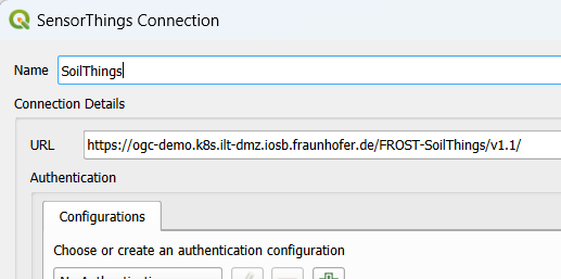
In the sources sidepanel, notice the option to add a Sensorthings API endpoint.
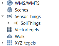
On Sensorthings panel, add the url to the service
Collapse the new service and notice a number of attribute and geometry tables which can be added to the Map View.
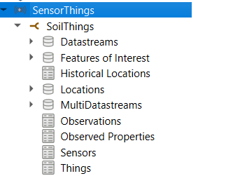
Add the features of interest to the map view. Open the attribute table (or select info from a single feature) and notice the information is quite limited. QGIS STA allows to expand the results of a single table with results from other tables.
Double click the layername in the Table of Contents and select the data source manager (source). Notice the ‘Expansions’ section and populate it with ‘Observations’, ‘Datastreams’, and ‘Observed properties’.
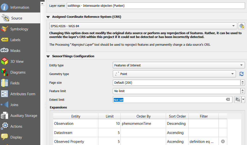
To prevent low performance, keep the pagination numbers (Limit) low. Also consider to add a filter on the Observed property to limit results to a single soil property.
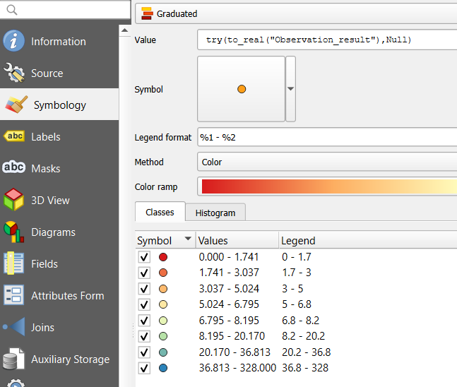
definition eq 'https://www.milieuinfo.be/confluence/x/S5vMC'Finally we want to colorise the map view based on the observation results. Double click the layername in TOC and select the symbology tab. Select a Graduated pattern based on an expression:
try(to_real("Observation_result"),Null)The Observation_result field is a string field. For that reason we add to_real() to force it to a number (and try() if conversion fails).
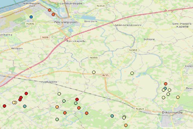
Which results in a nice map of texture observations in Belgium